Model Selection Strategy in Modern Panel Data Econometrics

One of the most common misconceptions in empirical research is that panel data analysis consists merely of choosing between Fixed Effects (FE) and Random Effects (RE) estimators. In reality, modern panel econometrics encompasses a broad family of estimators designed to address different violations of classical assumptions. Consequently, the central task of the researcher is not to select a model directly but to identify the characteristics of the underlying data-generating process (DGP) and then choose the estimator whose assumptions are most compatible with those characteristics.

The evolution of panel-data econometrics over the past three decades has largely been driven by the recognition that real-world datasets rarely satisfy the assumptions underlying traditional panel estimators. Cross-sectional units are often interconnected through common shocks, variables frequently exhibit stochastic trends, coefficients may differ across units, and explanatory variables are commonly endogenous. Each of these features gives rise to specific econometric problems that require specific methodological solutions. Therefore, model selection should be viewed as a process of progressively filtering out inappropriate estimators rather than identifying a single universally superior technique.

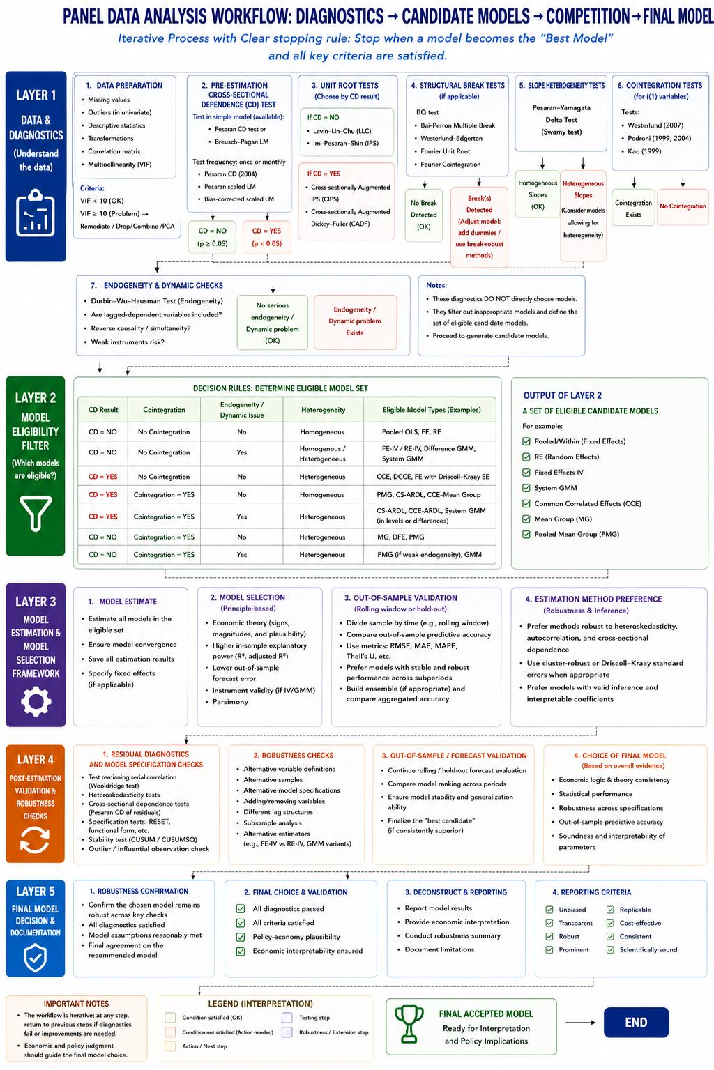
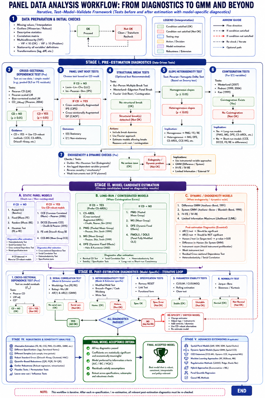
From this perspective, panel-data analysis proceeds through a hierarchy of questions. Are observations cross-sectionally independent? Are variables stationary? Do they share a long-run equilibrium relationship? Are coefficients homogeneous across units? Is endogeneity present? The answers to these questions gradually narrow the set of admissible estimators until a small number of theoretically and econometrically defensible models remain.

1. Static Panel Models as the Starting Point

The classical panel-data framework begins with pooled Ordinary Least Squares (OLS), Fixed Effects (FE), and Random Effects (RE) estimators. These models are often referred to as static panel estimators because they assume that current outcomes depend exclusively on contemporaneous explanatory variables and not on their own past realizations.

Pooled OLS represents the most restrictive specification because it assumes complete homogeneity across all cross-sectional units. Every unit is assumed to share identical intercepts and slope coefficients, implying that unobserved heterogeneity does not exist. Such an assumption is rarely plausible in economic applications involving countries, regions, firms, or households.

The Fixed Effects estimator relaxes this assumption by allowing each unit to possess its own time-invariant intercept. By eliminating unobserved heterogeneity through within-transformation, FE controls for omitted variables that remain constant over time. Consequently, FE is generally preferred whenever unobserved characteristics are correlated with explanatory variables.

The Random Effects estimator adopts a different strategy. Instead of eliminating unit-specific effects, RE treats them as random draws from a common distribution and assumes that they are uncorrelated with explanatory variables. Under this assumption, RE is more efficient than FE because it exploits both within-unit and between-unit variation. However, if the orthogonality assumption is violated, RE becomes inconsistent. The Hausman test therefore plays a central role in determining whether RE remains valid or whether FE should be preferred.

Although FE and RE remain indispensable tools, they were developed under assumptions that are increasingly difficult to justify in modern macro-panel datasets. In particular, they assume cross-sectional independence, slope homogeneity, and exogeneity of regressors. Once these assumptions are violated, more sophisticated estimators become necessary.

2. Cross-Sectional Dependence and the Rise of Second-Generation Panel Methods

A major breakthrough in panel econometrics emerged from the recognition that economic units are rarely independent. Countries are affected by global financial crises, regions respond to national policies, and firms face common technological shocks. These common influences generate cross-sectional dependence, meaning that disturbances become correlated across units.

The existence of cross-sectional dependence fundamentally changes the econometric environment. Traditional FE and RE estimators may continue to produce coefficient estimates, but standard errors become unreliable and asymptotic properties no longer hold. As a result, statistical inference may become severely distorted.

The Pesaran CD test is now widely regarded as the standard diagnostic tool for evaluating cross-sectional dependence. Once dependence is detected, the researcher faces a critical methodological transition. Rather than relying on conventional panel estimators, attention shifts toward Common Correlated Effects (CCE) estimators. The core insight underlying the CCE framework is that unobserved common factors can be approximated through cross-sectional averages of the dependent and explanatory variables.

Among these estimators, CCEMG allows both common shocks and coefficient heterogeneity, whereas DCCE extends the framework to dynamic settings. These approaches have become particularly important in macroeconomic and development studies because they explicitly recognize that countries and regions operate within interconnected economic systems rather than in isolation.

3. Stationarity, Unit Roots, and the Problem of Spurious Regression

The next stage of analysis concerns the time-series properties of the variables. Economic variables such as GDP, foreign direct investment, energy consumption, and trade openness frequently exhibit persistent trends over time. Estimating relationships among trending variables may generate statistically significant results even when no meaningful economic relationship exists.

This phenomenon, known as spurious regression, motivated the development of panel unit-root testing procedures. The objective of these tests is to determine whether fluctuations around long-run means occur or whether variables contain stochastic trends.

The distinction between first-generation and second-generation unit-root tests mirrors the distinction between independent and dependent cross-sections. First-generation tests, such as Levin-Lin-Chu (LLC) and Im-Pesaran-Shin (IPS), assume cross-sectional independence. Second-generation procedures, including CADF and CIPS tests, explicitly account for common factors.

The outcome of unit-root testing provides the foundation for all subsequent model-selection decisions. If variables are stationary, conventional panel estimators may be employed directly. If variables are integrated of order one, cointegration analysis becomes necessary.

4. Cointegration and Long-Run Equilibrium Modelling

Cointegration analysis emerged as a response to the observation that many economic variables are non-stationary yet move together over long periods. Economic theory frequently predicts such behavior. For example, income and trade openness may trend upward together, while financial development and economic growth often evolve within a common equilibrium framework.

Panel cointegration tests evaluate whether a stable long-run relationship exists among non-stationary variables. If cointegration is absent, long-run coefficient estimates become economically meaningless because variables drift independently over time. Under these circumstances, the researcher should focus on short-run models, often expressed in first differences.

The existence of cointegration dramatically alters the econometric strategy. Once a long-run equilibrium relationship is established, a family of estimators specifically designed for cointegrated panels becomes available. These include Dynamic Fixed Effects (DFE), Mean Group (MG), Pooled Mean Group (PMG), Fully Modified OLS (FMOLS), Dynamic OLS (DOLS), and more recently CS-ARDL and DCCE estimators.

The central distinction among these estimators concerns assumptions regarding long-run homogeneity. DFE imposes complete homogeneity on all coefficients. PMG allows heterogeneous short-run dynamics while constraining long-run coefficients to be identical. MG imposes no such restriction and estimates separate regressions for each cross-sectional unit before averaging the coefficients.

The choice among these estimators ultimately depends on whether economic theory supports common long-run effects and whether empirical tests reject slope homogeneity.

5. Parameter Heterogeneity and the Mean Group Revolution

Traditional panel estimators are built upon the assumption that all cross-sectional units respond similarly to changes in explanatory variables. This assumption is often unrealistic in international and regional studies. The effect of innovation on economic growth may differ substantially across countries with different institutional environments. Likewise, the growth impact of foreign direct investment may vary according to levels of human capital or technological capability.

The recognition of such heterogeneity led to the development of Mean Group estimators. Rather than imposing a common coefficient, MG estimates individual regressions for each unit and computes the average effect across units. This approach allows complete heterogeneity in both short-run and long-run responses.

The PMG estimator occupies an intermediate position between DFE and MG. It assumes that long-run relationships are common across units while permitting heterogeneous short-run adjustments. In many empirical applications, PMG is regarded as a compromise between efficiency and flexibility.

When cross-sectional dependence and heterogeneity coexist, estimators such as CCEMG and DCCE become particularly attractive because they simultaneously address both problems.

6. Endogeneity and Dynamic Panel Models

One of the most persistent challenges in empirical economics is endogeneity. Explanatory variables are frequently correlated with the error term due to omitted variables, simultaneity, reverse causality, or measurement error. In growth regressions, for example, innovation may stimulate growth while growth simultaneously stimulates innovation. Such feedback effects violate the exogeneity assumptions underlying FE and RE estimators.

Dynamic panel models provide a solution by incorporating lagged dependent variables and employing internal instruments. The seminal contributions of Arellano and Bond (1991), Arellano and Bover (1995), and Blundell and Bond (1998) gave rise to Difference GMM and System GMM estimators.

Difference GMM removes fixed effects through differencing and uses lagged levels as instruments. However, when variables are highly persistent, lagged levels become weak instruments. System GMM addresses this problem by combining equations in levels and differences, thereby improving efficiency and reducing finite-sample bias.

For panels characterized by large N and small T, System GMM is often regarded as the benchmark estimator when endogeneity is present. Nevertheless, its superiority should not be assumed automatically. GMM estimators are designed primarily to address endogeneity rather than cross-sectional dependence or long-run equilibrium relationships. Consequently, in datasets characterized by strong common factors and cointegration, CCE-based estimators or CS-ARDL may provide more reliable results than GMM.

7. Why CS-ARDL Has Become Increasingly Popular

Recent developments in panel econometrics have highlighted the limitations of traditional cointegration estimators when cross-sectional dependence is present. PMG, MG, and DFE were originally developed under assumptions that become questionable in highly interconnected economies.

CS-ARDL extends the ARDL framework by incorporating cross-sectional averages that proxy for unobserved common factors. As a result, it simultaneously addresses non-stationarity, cointegration, dynamic adjustment, cross-sectional dependence, and coefficient heterogeneity.

This combination of desirable properties explains the growing popularity of CS-ARDL in contemporary macroeconomic research. In many situations involving moderate or large time dimensions, CS-ARDL may be viewed as a natural extension of PMG into environments characterized by cross-sectional dependence.

For this reason, many recent studies increasingly adopt a strategy in which System GMM serves as the baseline estimator for dynamic endogeneity concerns, while CS-ARDL or DCCE estimators are employed as robustness checks designed to account for long-run dynamics and common factors.

8. Role of Sample Dimensions in Estimator Choice

The relative performance of panel estimators depends heavily on the dimensions of the dataset. The distinction between large-N/small-T and small-N/large-T panels remains one of the most important considerations in applied work.

Large-N/small-T panels are ideally suited for FE, RE, Difference GMM, and System GMM estimators. These methods were specifically developed under asymptotic frameworks where the number of cross-sectional units grows while the time dimension remains limited.

Small-N/large-T panels favor long-run estimators such as PMG, MG, DFE, CS-ARDL, DCCE, FMOLS, and DOLS. These estimators exploit rich time-series information to identify equilibrium relationships and dynamic adjustments.

When both N and T are large, researchers enjoy the greatest methodological flexibility. In such settings, advanced estimators capable of addressing multiple econometric problems simultaneously become feasible and often preferable.

9. Model Validation and the Iterative Nature of Econometric Analysis

The final stage of panel-data analysis involves model validation. Econometric modelling should not be viewed as a linear sequence ending with coefficient estimation. Instead, it is an iterative process in which diagnostic tests continually evaluate whether the chosen model remains consistent with the observed properties of the data.

Residual cross-sectional dependence suggests that common factors remain unmodelled. Serial correlation indicates dynamic misspecification. Heteroskedasticity affects statistical efficiency. Functional-form tests reveal omitted nonlinearities. Stability tests evaluate whether coefficients remain constant over time.

A model should only be accepted after successfully passing these diagnostic examinations. Failure of any diagnostic does not necessarily invalidate the entire analysis; rather, it signals that the specification must be revised and re-estimated. The preferred model is therefore not the one that generates the largest number of significant coefficients, but the one that remains theoretically coherent, statistically valid, and robust across alternative specifications.

From this perspective, modern panel econometrics is best understood as a process of progressively uncovering the structure of the data-generating mechanism. Diagnostics identify the relevant econometric challenges, estimators are selected to address those challenges, and post-estimation tests verify whether the chosen solution has been successful. The final model emerges not from convenience or popularity but from the convergence of economic theory, statistical evidence, and econometric validity.